How to Use and Interpret a Smith Chart

Understand how to use and interpret a Smith chart to help with RF design or using vector network analyzers

Home » Radio & RF technology » this page

Smith Charts Includes:
Smith chart basics How to use a Smith chart

The Smith chart is a very useful tool for investigating the impedance of a circuit. It is widely used by RF engineers and in RF test instruments.

Essentially, the Smith chart is a polar plot of the complex reflection coefficient, ρ, which is a measure of how much of a wave is reflected from a load impedance.

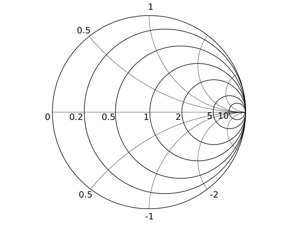
The Smith chart is a powerful tool for analysing and designing circuits at high frequencies, where the effects of transmission lines and other distributed components become significant.

The chart is also widely seen in one of the display modes for vector network analysers, VNSAs.

In view of its importance, the Smith chart is an essential for any RF engineer to master.

Key points of the Smith chart

When using the Smith chart there are a few key points to learn as these help with the understanding of the underlying principles and as a result it is possible to use it to the full:

The Centre is the match point

The very centre of the Smith Chart represents the system match point.

In most standard RF systems, this corresponds to a 50Ω reference impedance, although other systems may use different impedances. It is worth noting that the chart is normalised to the impedance being used. So that if a 50Ω impedance is being used, everything relates to this impedance.
When the system is perfectly matched to the reference impedance, the Voltage Standing Wave Ratio (VSWR) is exactly 1:1. This is the ultimate goal of impedance matching: bringing the impedance point exactly to the centre.

The Horizontal Axis: Real Resistance

The straight horizontal line cutting through the middle of the chart is the pure resistance axis.

Left Edge: Represents a **short circuit** (0\Omega, where voltage drops to zero).
Right Edge: Represents an **open circuit** (\infty\Omega, where current drops to zero).
Moving from left to right: Moving along this line transitions your load from zero resistance to infinite resistance.

Top and bottom sections: inductive vs. capacitive reactance

The curves bowing away from the horizontal axis represent imaginary reactance (j).

Top Half: This region represents **inductive reactance (+j)**. Any point plotted in the upper hemisphere contains an inductive component.
Bottom Half: This region represents **capacitive reactance (-j)**. Any point plotted in the lower hemisphere contains a capacitive component.

Constant VSWR Circles

If a perfect circle centred exactly at the match point is drawn, i.e. the centre of the chart, then these form constant VSWR circles.

The radius of this circle is directly proportional to the magnitude of the reflection coefficient (Γ). As a component is only altered in a way that only rotates around this centre point (like adding a lossless transmission line), the VSWR remains completely constant.

Navigating and reading the chart

Before plotting points, it is important to understand what normalisation is and how it is applied toth e chart.

Because a Smith Chart can be used for any system impedance, the chart uses normalised values, i.e they are related toth e impedance of the system being used: 50Ω for a 50Ω system and so forth.

To normalize an impedance, just divide the actual impedance (Z) by the system reference impedance (Z_0).

For example for a 50Ω system, an impedance of Z = 50 + j100Ω normalizes to z = 1 + j2.

Plotting a point

To find z = 1 + j2, you find the constant resistance circle marked **1** (which passes through the center of the chart) and follow it up into the top half until it intersects the constant reactance curve marked **2**.

Moving with series and shunt elements

Once the starting impedance is plotted, adding components alters the impedance, causing the the point on the chart to move across, along highly predictable paths:

Series Elements: When adding components in series, you move along the constant resistance circles.
Shunt (Parallel) Elements: When adding components in parallel, you move along the **constant conductance circles** (which are mirror images of the resistance circles, looping from the left edge instead of the right).

The rules of component movement

When manipulating impedance using lumped elements (inductors and capacitors), there are four fundamental movements:

Adding a Series Inductor:** Moves **clockwise** along a constant resistance circle (climbing into the inductive top half).
Adding a Series Capacitor:** Moves **counterclockwise** along a constant resistance circle (dropping into the capacitive bottom half).
Adding a Shunt Inductor:** Moves **counterclockwise** along a constant conductance circle.
Adding a Shunt Capacitor:** Moves **clockwise** along a constant conductance circle.

The effect of transmission lines

What happens when a length of transmission line is added to the load? A lossless transmission line does not add resistance or consume power; it merely changes the phase of the reflection coefficient.

Therefore, adding transmission line length rotates your plotted point clockwise toward the generator along a constant VSWR circle.