Butterworth Filter Formula, Equations, & Calculations

Whilst these days there are Apps and software to calculate filters like the Butterworth filter, the calculations can also be made manually.

Home » Radio & RF technology » this page

Butterworth Filter Includes:
Butterworth filter Butterworth calculations

Filter basics includes:: RF filters - the basics Filter specifications RF filter design basics High & low pass filter design Constant-k filter Butterworth filter Chebychev filter Bessel filter Elliptical filter

The Butterworth filter is a popular form of filter providing a maximally flat in-band response.Whilst the most common method of calculating the values these days is to use an app or other computer software, it is still possible calculate them using more traditional methods. There are formulas or equations that can be sued for these calculations and in this way it is possible to understand the trade-offs and workings more easily.

Using the equations for the Butterworth filter, it is relatively easy to calculate and plot the frequency response as well as working out the values needed.

Butterworth filter frequency response

As the Butterworth filter is maximally flat, this means that it is designed so that at zero frequency, the first 2n-1 derivatives for the power function with respect to frequency are zero.

Thus it is possible to derive the formula for the Butterworth filter frequency response:

{| \frac{V_{out}}{V_{in}} |}^{2} = \frac{1}{1 + {(\frac{f}{f_{c}})}^{2 n}}

Where:
   f = frequency at which calculation is made
   f_c = the cut-off frequency, i.e. half power or -3dB frequency
   Vin = input voltage
   Vout = output voltage
   n = number of elements in the filter

The equation can be re-written to give its more usual format. Here H(jω) is the transfer function and it is assumed the filter has no gain, i.e. it is not an active filter.

| H (j ω) | = \frac{1}{\sqrt{1 + {(\frac{ω}{ω_{c}})}^{2 n}}}

Where:
   H(jω) = transfer function at angular frequency ω
   ω = angular frequency and is equal to 2πf
   ω_c = cutoff frequency expressed as an angular value and is equal to 2πf_c

Note: It does not matter whether ω/ωo or f/f_c is used as it is purely a ratio of the two figures. If ω which is 2πf is used, then the factor 2π cancels out as it is on both the top and bottom of the fraction.

When wanting to express the loss of the Butterworth filter at any point, the Butterworth formula below can be used. This gives the attenuation in decibels at any point.

A_{d} = 10 \log_{10} (1 + {(\frac{ω}{ω_{c}})}^{2 n})

Butterworth filter calculation example

To provide an example of the response of the Butterworth filter calculation, take an example of the circuit given below. As is normal with these calculations normalised values are used where the cut-off frequency is 1 radian, i.e. 1/2Π Hz, the impedance is 1 Ω and values are given in Farads and Henries.

The example below uses some of the simplest values, with an impedance of 1Ω, and values for the capacitor of 2 Farads and the series inductors each 1 Henry.

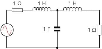
Using the formula above and a knowledge of the cut-off point being 0.159Hz, it is possible to calculate values of response at various frequencies:

Response of Butterworth Filter
Frequency (Hz)	Relative Power Output
0.00	1.00
0.07	0.99
0.095	0.95
0.159	0.50
0.223	0.117
0.254	0.056
0.318	0.015

Butterworth filter poles

The poles of a Butterworth low-pass filter with cut-off frequency ωc are evenly-spaced around the circumference of a half-circle of radius ωc centred upon the origin of the s-plane.

The poles of a two-pole filter are at ±45°. Those of a four-pole filter are at ±22.5° and ±67.5°. Other cases can also be deduced in a similar fashion.

However the table below provides the poles of the low-pass Butterworth filters with one to eight poles and cut-off frequency 1 rad/s, i.e. for a normalised filter.

Poles of the Normalized Butterworth Polynomials
Order	Poles
1	−1 ± j 0
2	−0.707 ± j 0.707
3	−1 ± j 0, −0.5 ± j 0.866
4	−0.924 ± j 0.383, −0.383 ± j 0.924
5	−1 ± j 0, −0.809 ± j 0.588, −0.309 ± j 0.951
6	−0.966 ± j 0.259, −0.707 ± j 0.707, −0.259 ± j 0.966
7	−1 ± j 0, −0.901 ± j 0.434, −0.624 ± j 0.782, −0.222 ± j 0.975
8	−0.981 ± j 0.195, −0.832 ± j 0.556, −0.556 ± j 0.832, −0.195 ± j 0.981